Comparison of Preranked Gene Set Enrichment analysis(GSEA), traditional GSEA and fGSEA in Python and R
Author: Shakira Agata
This Jupyter notebook describes the steps for the execution and comparison of methods: preranked GSEA, traditional GSEA and fGSEA (Fast Gene Set Enrichment Analysis). My goal was to identify the potential difference in outcomes when using three different methods of GSEA: preranked GSEA from GSEApy, traditional GSEA from GSEApy and fGSEA from Bioconductor(1,2). I did this by comparing the outcomes in identified pathways, calculated Enrichment Scores (ES) and Normalized Enrichment Scores for the three methods. The comparison was made using the data for Ag+ and control at 24 hours from ArrayExpress dataset: E-MEXP-3583. This dataset looked at the effect of Ag+ and AgNPs on the gene expression in a human lung epithelial cell line A549.
This notebook is subdivided into the following two sections:
Section 1: Preranked GSEA
Section 1.1: System preparation
Section 1.2: Generation of the RNK file
Section 1.3: Selection of the geneset
Section 1.4: Execution of GSEA
Section 2: Traditional GSEA
Section 2.1: Generation of expression data frame
Section 2.2: Generation of the CLS file
Section 2.3: Selection of the geneset
Section 2.4: Execution of GSEA
Section 3: fGSEA
Section 3.1 Magic R extension and system preparation
Section 3.2 Execution of fGSEA
Section 4: Session information for Python and R
Section 4.1: Python session information
Section 4.2: R session information
Section 1: Preranked GSEA
In this section, the preranked GSEA method will be used which allows users to select the ranking method for the comparison of two group of samples (e.g control and treatment). In this case, the differential gene expression results for the comparison of Ag+ to the control at 24h was used to allow for the calculation of the ranking by the log2FC. This ranking method is used in the formal documentation of GSEA and can be used as option in fGSEA and Clusterprofiler GSEA in Rstudio (1).
Section 1.1: System preparation
Step 1. The necessary packages for using this pipeline are first installed.
[6]:
import pandas as pd
from gseapy.plot import gseaplot
import gseapy as gp
import numpy as np
import matplotlib.pyplot as plt
from gseapy import dotplot
[7]:
pip install watermark
Requirement already satisfied: watermark in c:\users\shaki\anaconda3\lib\site-packages (2.4.3)
Requirement already satisfied: ipython>=6.0 in c:\users\shaki\anaconda3\lib\site-packages (from watermark) (8.25.0)
Requirement already satisfied: importlib-metadata>=1.4 in c:\users\shaki\anaconda3\lib\site-packages (from watermark) (7.0.1)
Requirement already satisfied: setuptools in c:\users\shaki\anaconda3\lib\site-packages (from watermark) (69.5.1)
Requirement already satisfied: zipp>=0.5 in c:\users\shaki\anaconda3\lib\site-packages (from importlib-metadata>=1.4->watermark) (3.17.0)
Requirement already satisfied: decorator in c:\users\shaki\anaconda3\lib\site-packages (from ipython>=6.0->watermark) (5.1.1)
Requirement already satisfied: jedi>=0.16 in c:\users\shaki\anaconda3\lib\site-packages (from ipython>=6.0->watermark) (0.18.1)
Requirement already satisfied: matplotlib-inline in c:\users\shaki\anaconda3\lib\site-packages (from ipython>=6.0->watermark) (0.1.6)
Requirement already satisfied: prompt-toolkit<3.1.0,>=3.0.41 in c:\users\shaki\anaconda3\lib\site-packages (from ipython>=6.0->watermark) (3.0.43)
Requirement already satisfied: pygments>=2.4.0 in c:\users\shaki\anaconda3\lib\site-packages (from ipython>=6.0->watermark) (2.15.1)
Requirement already satisfied: stack-data in c:\users\shaki\anaconda3\lib\site-packages (from ipython>=6.0->watermark) (0.2.0)
Requirement already satisfied: traitlets>=5.13.0 in c:\users\shaki\anaconda3\lib\site-packages (from ipython>=6.0->watermark) (5.14.3)
Requirement already satisfied: colorama in c:\users\shaki\anaconda3\lib\site-packages (from ipython>=6.0->watermark) (0.4.6)
Requirement already satisfied: parso<0.9.0,>=0.8.0 in c:\users\shaki\anaconda3\lib\site-packages (from jedi>=0.16->ipython>=6.0->watermark) (0.8.3)
Requirement already satisfied: wcwidth in c:\users\shaki\anaconda3\lib\site-packages (from prompt-toolkit<3.1.0,>=3.0.41->ipython>=6.0->watermark) (0.2.5)
Requirement already satisfied: executing in c:\users\shaki\anaconda3\lib\site-packages (from stack-data->ipython>=6.0->watermark) (0.8.3)
Requirement already satisfied: asttokens in c:\users\shaki\anaconda3\lib\site-packages (from stack-data->ipython>=6.0->watermark) (2.0.5)
Requirement already satisfied: pure-eval in c:\users\shaki\anaconda3\lib\site-packages (from stack-data->ipython>=6.0->watermark) (0.2.2)
Requirement already satisfied: six in c:\users\shaki\anaconda3\lib\site-packages (from asttokens->stack-data->ipython>=6.0->watermark) (1.16.0)
Note: you may need to restart the kernel to use updated packages.
[notice] A new release of pip is available: 24.3.1 -> 25.0.1
[notice] To update, run: python.exe -m pip install --upgrade pip
Section 1.2: Generation of the RNK file
Step 2. Next, you load the data from E-MEXP3583 into a dataframe.
[10]:
df1 = pd.read_csv('topTable_Ag._.1.3_24 - H2O.control_.0.0_24-try.csv').dropna()
df1
[10]:
| GeneID | meanExpr | log2FC | log2FC SE | p-value | adjpvalue | |
|---|---|---|---|---|---|---|
| 0 | 4490 | 9.925881 | 3.935193 | 0.206737 | 9.842270e-11 | 0.000002 |
| 1 | 4495 | 9.561522 | 4.109887 | 0.243653 | 3.924060e-10 | 0.000004 |
| 2 | 79974 | 6.381454 | 2.532636 | 0.174021 | 2.094514e-09 | 0.000011 |
| 3 | 4489 | 12.843381 | 2.498127 | 0.172052 | 2.150589e-09 | 0.000011 |
| 4 | 1638 | 6.429810 | 2.349836 | 0.170834 | 3.954792e-09 | 0.000016 |
| ... | ... | ... | ... | ... | ... | ... |
| 20513 | 391257 | 6.462645 | -0.000055 | 0.146291 | 9.996750e-01 | 0.999870 |
| 20514 | 10078 | 8.351476 | -0.000037 | 0.128166 | 9.997478e-01 | 0.999894 |
| 20515 | 84328 | 9.130185 | -0.000033 | 0.167015 | 9.998260e-01 | 0.999923 |
| 20516 | 253018 | 7.162925 | -0.000015 | 0.199487 | 9.999336e-01 | 0.999982 |
| 20517 | 440737 | 10.365751 | 0.000003 | 0.187502 | 9.999848e-01 | 0.999985 |
20518 rows × 6 columns
Step 3. The dataframe is reformatted so that the geneID and log2FC columns are kept. In this case, the log2FC used as the rank and thus the name of the column:log2FC is changed to ‘Rank’.
[12]:
df2= df1[['GeneID','log2FC']]
df3= df2.rename(columns={'log2FC':'Rank'})
df3
[12]:
| GeneID | Rank | |
|---|---|---|
| 0 | 4490 | 3.935193 |
| 1 | 4495 | 4.109887 |
| 2 | 79974 | 2.532636 |
| 3 | 4489 | 2.498127 |
| 4 | 1638 | 2.349836 |
| ... | ... | ... |
| 20513 | 391257 | -0.000055 |
| 20514 | 10078 | -0.000037 |
| 20515 | 84328 | -0.000033 |
| 20516 | 253018 | -0.000015 |
| 20517 | 440737 | 0.000003 |
20518 rows × 2 columns
Step 4. The datatype of the first column of df3 is changed to a string as needed for the GSEA function we will use in section 1.4. The ‘Rank’ column will remain unnchanged as rank needs to remain numeric for the GSEA function. We also remove duplicates as duplicates will raise errors when running GSEA.
[14]:
df3['GeneID']=df3['GeneID'].astype(str)
ranking=df3.drop_duplicates(subset="GeneID", keep="first")
Section 1.3 Selection of the geneset
Step 5. Here, you can select the geneset of interest. The command below displays the available options. In this notebook, the ENTREZ ID version of WikiPathways 2024 Human will be used.
[17]:
names = gp.get_library_name()
Section 1.4: Execution of preranked GSEA
Step 6. Preranked GSEA can be executed by selection of the RNK file and gene set. The seed, min_size, max_size and permutation number were set to those below in accordance with the formal documentation of GSEAPY. The permutation type was set to ‘gene_set’ as we have less than 15 samples and verbose was set to TRUE to get more insight into the GSEA process(1).
[20]:
Preranked_GSEA= gp.prerank(rnk=ranking,
                     gene_sets='c2.cp.wikipathways.v2024.1.Hs.entrez.gmt',
                     min_size=5,
                     max_size=1000,
                     permutation_type='gene_set',
                     seed=6,
                     permutation_num=1000,
                     verbose=True)
2025-03-04 11:19:47,130 [INFO] Parsing data files for GSEA.............................
2025-03-04 11:19:47,195 [INFO] 0000 gene_sets have been filtered out when max_size=1000 and min_size=5
2025-03-04 11:19:47,195 [INFO] 0830 gene_sets used for further statistical testing.....
2025-03-04 11:19:47,199 [INFO] Start to run GSEA...Might take a while..................
2025-03-04 11:20:38,521 [INFO] Congratulations. GSEApy runs successfully................
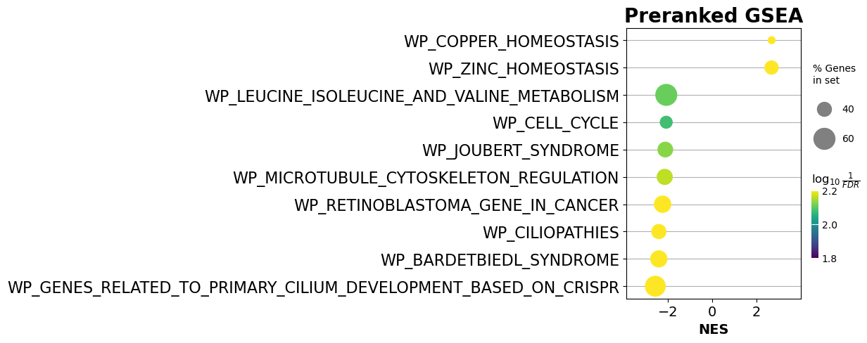
Step 7. In the next step, the results are displayed and visualized.
[22]:
Preranked_GSEA.res2d.head(5)
[22]:
| Name | Term | ES | NES | NOM p-val | FDR q-val | FWER p-val | Tag % | Gene % | Lead_genes | |
|---|---|---|---|---|---|---|---|---|---|---|
| 0 | prerank | WP_COPPER_HOMEOSTASIS | 0.758562 | 2.676049 | 0.0 | 0.0 | 0.0 | 12/53 | 2.46% | 4495;4490;4501;4489;4494;4496;4493;84560;4500;... |
| 1 | prerank | WP_ZINC_HOMEOSTASIS | 0.816562 | 2.670822 | 0.0 | 0.0 | 0.0 | 15/37 | 5.27% | 4495;4490;4501;4489;4494;7780;4496;7779;4493;8... |
| 2 | prerank | WP_GENES_RELATED_TO_PRIMARY_CILIUM_DEVELOPMENT... | -0.546802 | -2.576323 | 0.0 | 0.0 | 0.0 | 60/101 | 27.17% | 55764;8100;132320;23322;57539;23059;79659;5508... |
| 3 | prerank | WP_BARDETBIEDL_SYNDROME | -0.540727 | -2.417239 | 0.0 | 0.0 | 0.0 | 42/86 | 20.25% | 55764;132320;2736;5311;5727;57539;23059;79659;... |
| 4 | prerank | WP_CILIOPATHIES | -0.470576 | -2.415103 | 0.0 | 0.0 | 0.0 | 78/181 | 20.38% | 1063;55764;132320;4751;2736;5311;4867;219844;2... |
[23]:
ax1 = dotplot(Preranked_GSEA.res2d,
             column="FDR q-val",
             title='Preranked GSEA',
             cmap=plt.cm.viridis,
             size=6, # adjust dot size
             figsize=(4,5), cutoff=0.25, show_ring=False)
C:\Users\shaki\anaconda3\Lib\site-packages\gseapy\plot.py:738: FutureWarning: Downcasting behavior in `replace` is deprecated and will be removed in a future version. To retain the old behavior, explicitly call `result.infer_objects(copy=False)`. To opt-in to the future behavior, set `pd.set_option('future.no_silent_downcasting', True)`
  df[self.colname] = df[self.colname].replace(0, np.nan).bfill()
Section 2: Traditional GSEA
In this section, traditional GSEA will be executed. This method allows for 5 ranking methods including: signal_to_noise, t_test, ratio_of_classes, diff_of_classes and log2_ratio_of_classes. In order to use this method, the following two files have to be prepared beforehand.
Section 2.1 Generation of expression data frame
Step 8. Gene expression data dataframe will be generated in this step. The gene expression data file is a expression value table in which the sample names are placed horizontal and the gene names are placed vertical. This data was loaded and manipulated to meet GSEA guidelines.
[28]:
df= pd.read_csv('TraditionalGSEA-EMEXP3583.csv')
df.to_csv('TraditionalGSEA-EMEXP3583-version2.txt', sep='\t',index=False)
df2 = pd.read_csv("TraditionalGSEA-EMEXP3583-version2.txt",sep="\t", index_col=0)
df2 = df2.loc[:, ['M225-05', 'M225-01L', 'M225-03','M225-07']]
TraditionalGSEA= df2.rename(columns={"M225-05": "Control", "M225-01L": "Control","M225-03": "Treatment","M225-07": "Treatment"})
[29]:
TraditionalGSEA
[29]:
| Control | Control | Treatment | Treatment | |
|---|---|---|---|---|
| EntrezID | ||||
| 1 | 7.941181 | 8.006905 | 7.990053 | 8.326014 |
| 10 | 4.473060 | 4.561733 | 4.546220 | 4.573649 |
| 100 | 10.246258 | 10.481636 | 10.297045 | 10.176861 |
| 1000 | 11.149919 | 11.145671 | 11.090569 | 11.116654 |
| 10000 | 10.274072 | 10.243285 | 10.226056 | 10.054899 |
| ... | ... | ... | ... | ... |
| 9991 | 10.900741 | 10.551433 | 10.444575 | 10.473755 |
| 9992 | 5.068302 | 5.348781 | 5.664488 | 5.512333 |
| 9993 | 9.888579 | 10.014469 | 9.710480 | 9.798821 |
| 9994 | 7.720305 | 7.575626 | 7.660303 | 7.523620 |
| 9997 | 8.247325 | 8.484476 | 8.669681 | 8.838813 |
20518 rows × 4 columns
Section 2.2 Generation of the CLS file
Step 9. The CLS file was created according to the GSEA guidelines. Based on the expression data, the following structure of the cls file was created and saved with a cls extension:
CLS file structure:
First line : 4 2 1
Second line: # Control Treatment
Third line: ‘Control’ ‘Control’ ‘Treatment’ ‘Treatment’
[32]:
with open("clsfile.cls", "w") as file:
    file.write("4 2 1\n")
    file.write("# Control Treatment \n")
    file.write("'Control' 'Control' 'Treatment' 'Treatment'\n")
Section 2.3 Selection of the geneset
In this section, the geneset of interest can be selected. In this notebook, the ENTREZ ID version of WikiPathways 2024 Human will be used.
Section 2.4 Execution of traditional GSEA
Step 10. Lastly traditional GSEA was executed. This requires setting the EntrezID as the index and maintenance of the same parameters as for preranked GSEA.
[37]:
TraditionalGSEA.reset_index('EntrezID', inplace=True)
[38]:
TraditionalGSEA['EntrezID'] = TraditionalGSEA['EntrezID'].astype(str)
[39]:
GSEA = gp.gsea(data=TraditionalGSEA,
                 gene_sets='c2.cp.wikipathways.v2024.1.Hs.entrez.gmt',
                 cls= "clsfile.cls",
                 min_size=5,
                 max_size=1000,
                 permutation_num=1000,
                 permutation_type='gene_set',
                 outdir=None,
                 method='log2_ratio_of_classes',
                 threads=4,
                 verbose=True,
                 seed= 6)
2025-03-04 11:20:41,812 [INFO] Parsing data files for GSEA.............................
2025-03-04 11:20:41,887 [INFO] 0000 gene_sets have been filtered out when max_size=1000 and min_size=5
2025-03-04 11:20:41,887 [INFO] 0830 gene_sets used for further statistical testing.....
2025-03-04 11:20:41,887 [INFO] Start to run GSEA...Might take a while..................
2025-03-04 11:21:42,060 [INFO] Congratulations. GSEApy ran successfully.................
[40]:
print(GSEA.res2d.head())
   Name                                               Term        ES  \
0  gsea  WP_GENES_RELATED_TO_PRIMARY_CILIUM_DEVELOPMENT...  0.557377
1  gsea                                WP_ZINC_HOMEOSTASIS -0.775016
2  gsea                            WP_BARDETBIEDL_SYNDROME   0.50323
3  gsea                              WP_COPPER_HOMEOSTASIS -0.696479
4  gsea  WP_REGULATION_OF_SISTER_CHROMATID_SEPARATION_A...  0.720957

        NES NOM p-val FDR q-val FWER p-val   Tag %  Gene %  \
0  2.580045       0.0       0.0        0.0  50/101  21.25%
1 -2.319458       0.0       0.0        0.0   13/37   4.76%
2  2.290378       0.0  0.002076      0.002   40/86  19.31%
3  -2.19289       0.0       0.0        0.0   12/53   7.55%
4  2.130938       0.0  0.020764      0.029    4/14   4.81%

                                          Lead_genes
0  8100;55764;132320;23322;79659;57539;23059;1328...
1  4495;4490;4501;4489;7780;4496;4494;4493;84560;...
2  55764;132320;79659;2736;57539;5311;23059;13288...
3  4495;4490;4501;4489;4496;4494;4493;84560;4500;...
4                                 1062;9232;9700;699
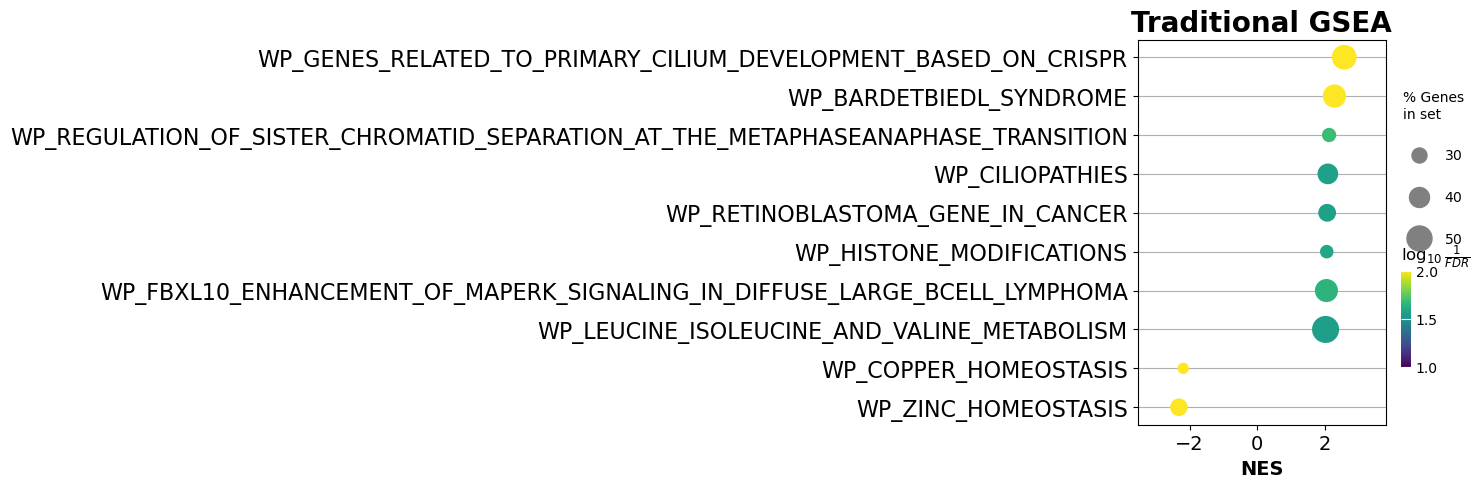
Step 11. In the next step, the results are displayed and visualized.
[42]:
ax2 = dotplot(GSEA.res2d,
             column="FDR q-val",
             title='Traditional GSEA',
             cmap=plt.cm.viridis,
             size=6, # adjust dot size
             figsize=(4,5), cutoff=0.25, show_ring=False)
C:\Users\shaki\anaconda3\Lib\site-packages\gseapy\plot.py:738: FutureWarning: Downcasting behavior in `replace` is deprecated and will be removed in a future version. To retain the old behavior, explicitly call `result.infer_objects(copy=False)`. To opt-in to the future behavior, set `pd.set_option('future.no_silent_downcasting', True)`
  df[self.colname] = df[self.colname].replace(0, np.nan).bfill()
Section 3: fGSEA
In this section, fast GSEA (fGSEA) will be executed which is a package developed by BioConductor. To be able to use this package in this notebook, rpy2 was employed.
Section 3.1 Magic R extension and system preparation
Step 12. We first activate rpy2 in this notebook. If a Windows laptop is used, the the warning ‘quartz’ may appear which can be ignored.
[47]:
%load_ext rpy2.ipython
C:\Users\shaki\anaconda3\Lib\site-packages\rpy2\robjects\packages.py:367: UserWarning: The symbol 'quartz' is not in this R namespace/package.
  warnings.warn(
Step 13. Next, the needed packages for fGSEA are installed. Dpending on the user’s background and possible prior experience with R, notifications for updating packages may appear. These notifications can be answered at users discretion.
[49]:
%%R
if (!require("BiocManager", quietly = TRUE))
    install.packages("BiocManager")

BiocManager::install("clusterProfiler")
R[write to console]: Bioconductor version 3.20 (BiocManager 1.30.25), R 4.4.1 (2024-06-14 ucrt)

R[write to console]: Bioconductor version 3.20 (BiocManager 1.30.25), R 4.4.1 (2024-06-14 ucrt)

R[write to console]: Installation paths not writeable, unable to update packages
  path: C:/Program Files/R/R-4.4.1/library
  packages:
    class, cluster, foreign, KernSmooth, Matrix, nlme, nnet, rpart, spatial,
    survival

R[write to console]: Old packages: 'aplot', 'Biostrings', 'cli', 'cpp11', 'ggnewscale', 'igraph',
  'IRanges', 'jsonlite', 'MASS', 'processx', 'R.utils', 'readxl', 'recolorize',
  'rlang', 'S4Vectors', 'terra', 'tinytex', 'xml2', 'XVector', 'zlibbioc'
Update all/some/none? [a/s/n]:
n
[50]:
%%R
if (!require("BiocManager", quietly = TRUE))
    install.packages("BiocManager")

BiocManager::install("fgsea")
R[write to console]: Bioconductor version 3.20 (BiocManager 1.30.25), R 4.4.1 (2024-06-14 ucrt)

R[write to console]: Installation paths not writeable, unable to update packages
  path: C:/Program Files/R/R-4.4.1/library
  packages:
    class, cluster, foreign, KernSmooth, Matrix, nlme, nnet, rpart, spatial,
    survival

R[write to console]: Old packages: 'aplot', 'Biostrings', 'cli', 'cpp11', 'ggnewscale', 'igraph',
  'IRanges', 'jsonlite', 'MASS', 'processx', 'R.utils', 'readxl', 'recolorize',
  'rlang', 'S4Vectors', 'terra', 'tinytex', 'xml2', 'XVector', 'zlibbioc'
Update all/some/none? [a/s/n]:
n
[51]:
%%R
install.packages(c ("readr","ggplot2","data.table","dplyr"))
R[write to console]: Installing packages into 'C:/Users/shaki/AppData/Local/R/win-library/4.4'
(as 'lib' is unspecified)
--- Please select a CRAN mirror for use in this session ---
R[write to console]: trying URL 'https://mirror.lyrahosting.com/CRAN/bin/windows/contrib/4.4/readr_2.1.5.zip'

R[write to console]: Content type 'application/zip'
R[write to console]:  length 1223048 bytes (1.2 MB)

R[write to console]: downloaded 1.2 MB


R[write to console]: trying URL 'https://mirror.lyrahosting.com/CRAN/bin/windows/contrib/4.4/ggplot2_3.5.1.zip'

R[write to console]: Content type 'application/zip'
R[write to console]:  length 5021782 bytes (4.8 MB)

R[write to console]: downloaded 4.8 MB


R[write to console]: trying URL 'https://mirror.lyrahosting.com/CRAN/bin/windows/contrib/4.4/data.table_1.17.0.zip'

R[write to console]: Content type 'application/zip'
R[write to console]:  length 2910072 bytes (2.8 MB)

R[write to console]: downloaded 2.8 MB


R[write to console]: trying URL 'https://mirror.lyrahosting.com/CRAN/bin/windows/contrib/4.4/dplyr_1.1.4.zip'

R[write to console]: Content type 'application/zip'
R[write to console]:  length 1590307 bytes (1.5 MB)

R[write to console]: downloaded 1.5 MB
package 'readr' successfully unpacked and MD5 sums checked
R[write to console]: Warning:
R[write to console]:  cannot remove prior installation of package 'readr'

R[write to console]: Warning:
R[write to console]:  restored 'readr'
package 'ggplot2' successfully unpacked and MD5 sums checked
package 'data.table' successfully unpacked and MD5 sums checked
R[write to console]: Warning:
R[write to console]:  cannot remove prior installation of package 'data.table'

R[write to console]: Warning:
R[write to console]:  restored 'data.table'
package 'dplyr' successfully unpacked and MD5 sums checked
R[write to console]: Warning:
R[write to console]:  cannot remove prior installation of package 'dplyr'

R[write to console]: Warning:
R[write to console]:  restored 'dplyr'
The downloaded binary packages are in
        C:\Users\shaki\AppData\Local\Temp\RtmpYdIkNC\downloaded_packages
Step 14. Next, the installed libraries are loaded prior to use.
[53]:
%%R
library(fgsea)
library(ggplot2)
library(data.table)
library(readr)
library(clusterProfiler)
library(dplyr)
R[write to console]: data.table 1.17.0 using 4 threads (see ?getDTthreads).
R[write to console]: Latest news: r-datatable.com

R[write to console]:

R[write to console]: clusterProfiler v4.14.6 Learn more at https://yulab-smu.top/contribution-knowledge-mining/

Please cite:

S Xu, E Hu, Y Cai, Z Xie, X Luo, L Zhan, W Tang, Q Wang, B Liu, R Wang,
W Xie, T Wu, L Xie, G Yu. Using clusterProfiler to characterize
multiomics data. Nature Protocols. 2024, 19(11):3292-3320

R[write to console]:
Attaching package: 'clusterProfiler'


R[write to console]: The following object is masked from 'package:stats':

    filter


R[write to console]:
Attaching package: 'dplyr'


R[write to console]: The following objects are masked from 'package:data.table':

    between, first, last


R[write to console]: The following objects are masked from 'package:stats':

    filter, lag


R[write to console]: The following objects are masked from 'package:base':

    intersect, setdiff, setequal, union
Section 3.2 Execution of fGSEA
Step 15. fGSEA can be executed by first loading the data. At this step, the rankData variable name will be created which contains the GeneID and log2FC column of data.
[56]:
%%R
data <- read_csv('topTable_Ag._.1.3_24 - H2O.control_.0.0_24-try.csv',show_col_types = FALSE)
rankData <- data$log2FC
names(rankData) <- data$GeneID
head(rankData)
    4490     4495    79974     4489     1638     4501
3.935193 4.109887 2.532636 2.498127 2.349836 2.727981
Step 16. Next, the geneset of interest is read into the variable name: ‘pathway’.
[58]:
%%R
pathway <- gmtPathways("./c2.cp.wikipathways.v2024.1.Hs.entrez.gmt")
Step 17. Lastly, fgGSEA is run and results are displayed. Based on the NES and ES scores, we can see strong similarity to the values observed for the preranked GSEA.
[60]:
%%R
fgseaRes <- fgseaMultilevel(pathway,
                  rankData,
                  minSize=10,
                  maxSize = 500)

fgseaRes %>%
  arrange(desc(abs(NES))) %>%
  top_n(10, -padj)
                                                           pathway         pval
                                                            <char>        <num>
 1:                                          WP_COPPER_HOMEOSTASIS 1.537901e-12
 2:                                            WP_ZINC_HOMEOSTASIS 5.055497e-13
 3: WP_GENES_RELATED_TO_PRIMARY_CILIUM_DEVELOPMENT_BASED_ON_CRISPR 1.766840e-11
 4:                                        WP_BARDETBIEDL_SYNDROME 2.574977e-09
 5:                                                WP_CILIOPATHIES 8.496336e-13
 6:                               WP_RETINOBLASTOMA_GENE_IN_CANCER 4.165935e-07
 7:                                            WP_JOUBERT_SYNDROME 3.479830e-06
 8:                                                  WP_CELL_CYCLE 4.005527e-07
 9:                                           WP_CILIARY_LANDSCAPE 1.492812e-08
10:       WP_OVERVIEW_OF_PROINFLAMMATORY_AND_PROFIBROTIC_MEDIATORS 2.309469e-05
            padj   log2err         ES       NES  size  leadingEdge
           <num>     <num>      <num>     <num> <int>       <list>
 1: 3.649953e-10 0.9101197  0.7585618  2.699857    53 4495, 44....
 2: 3.024696e-10 0.9214260  0.8165622  2.665558    37 4495, 44....
 3: 3.144975e-09 0.8634154 -0.5468024 -2.521632   101 55764, 8....
 4: 3.666768e-07 0.7749390 -0.5407270 -2.449247    86 55764, 1....
 5: 3.024696e-10 0.9214260 -0.4705761 -2.370628   181 1063, 55....
 6: 3.707682e-05 0.6749629 -0.4887608 -2.226432    87 891, 241....
 7: 2.752932e-04 0.6272567 -0.4782106 -2.104594    76 4646, 48....
 8: 3.707682e-05 0.6749629 -0.4340094 -2.068247   119 891, 534....
 9: 1.771470e-06 0.7337620 -0.3807739 -1.945516   210 3934, 55....
10: 1.644342e-03 0.5756103  0.4737143  1.925449   124 6375, 63....
[61]:
%%R

topPathwaysUp <- fgseaRes[ES > 0][head(order(pval), n=10), pathway]
topPathwaysDown <- fgseaRes[ES < 0][head(order(pval), n=10), pathway]
topPathways <- c(topPathwaysUp, rev(topPathwaysDown))
plotGseaTable(pathway[topPathways], rankData, fgseaRes, gseaParam=0.5)
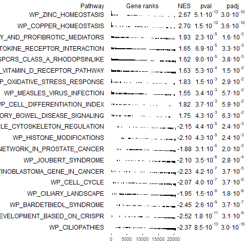
Conclusion: Using both methods of GSEA in GSEApy revealed that the ranking method affects the pattern in NES scores. Besides the debate on the best ranking method, the internal ranking in the traditional GSEA yields a different pattern compared to the explicit usage of log2FC in preranked GSEA. To further confirm the findings, fGSEA was executed which yielded NES scores and ES scores similar to preranked GSEA. The usage of logFC explicitly in preranked GSEA appears more in line with findings from other GSEA packages and descriptions of GSEA tutorials.
Section 4. Session information for Python and R
In this section, the session information for both Python and R used in this notebook will be displayed.
Section 4.1: Python session information
[66]:
%load_ext watermark
%watermark
Last updated: 2025-03-04T11:33:17.306769+01:00

Python implementation: CPython
Python version       : 3.12.3
IPython version      : 8.25.0

Compiler    : MSC v.1938 64 bit (AMD64)
OS          : Windows
Release     : 11
Machine     : AMD64
Processor   : Intel64 Family 6 Model 140 Stepping 1, GenuineIntel
CPU cores   : 8
Architecture: 64bit
Section 4.2: R session information
[68]:
%%R
sessionInfo()
R version 4.4.1 (2024-06-14 ucrt)
Platform: x86_64-w64-mingw32/x64
Running under: Windows 11 x64 (build 26100)

Matrix products: default


locale:
[1] LC_COLLATE=Dutch_Netherlands.1252  LC_CTYPE=Dutch_Netherlands.1252
[3] LC_MONETARY=Dutch_Netherlands.1252 LC_NUMERIC=C
[5] LC_TIME=Dutch_Netherlands.1252

time zone: Europe/Amsterdam
tzcode source: internal

attached base packages:
[1] tools     stats     graphics  grDevices utils     datasets  methods
[8] base

other attached packages:
[1] dplyr_1.1.4            clusterProfiler_4.14.6 readr_2.1.5
[4] data.table_1.17.0      ggplot2_3.5.1          fgsea_1.32.2
[7] BiocManager_1.30.25

loaded via a namespace (and not attached):
 [1] tidyselect_1.2.1        farver_2.1.2            blob_1.2.4
 [4] R.utils_2.12.3          Biostrings_2.73.2       lazyeval_0.2.2
 [7] fastmap_1.2.0           digest_0.6.37           lifecycle_1.0.4
[10] KEGGREST_1.46.0         tidytree_0.4.6          RSQLite_2.3.9
[13] magrittr_2.0.3          compiler_4.4.1          rlang_1.1.4
[16] igraph_2.1.3            ggtangle_0.0.6          labeling_0.4.3
[19] bit_4.5.0.1             gson_0.1.0              plyr_1.8.9
[22] RColorBrewer_1.1-3      aplot_0.2.4             BiocParallel_1.40.0
[25] purrr_1.0.4             withr_3.0.2             BiocGenerics_0.52.0
[28] R.oo_1.27.0             grid_4.4.1              stats4_4.4.1
[31] GOSemSim_2.32.0         enrichplot_1.26.6       colorspace_2.1-1
[34] GO.db_3.20.0            scales_1.3.0            cli_3.6.3
[37] crayon_1.5.3            treeio_1.30.0           generics_0.1.3
[40] ggtree_3.14.0           httr_1.4.7              reshape2_1.4.4
[43] tzdb_0.4.0              ape_5.8-1               DBI_1.2.3
[46] qvalue_2.38.0           cachem_1.1.0            DOSE_4.0.0
[49] stringr_1.5.1           zlibbioc_1.51.2         splines_4.4.1
[52] parallel_4.4.1          ggplotify_0.1.2         AnnotationDbi_1.68.0
[55] XVector_0.45.0          vctrs_0.6.5             yulab.utils_0.2.0
[58] Matrix_1.7-1            jsonlite_1.8.9          gridGraphics_0.5-1
[61] IRanges_2.39.2          hms_1.1.3               patchwork_1.3.0
[64] S4Vectors_0.43.2        ggrepel_0.9.6           bit64_4.6.0-1
[67] tidyr_1.3.1             snow_0.4-4              glue_1.8.0
[70] codetools_0.2-20        cowplot_1.1.3           stringi_1.8.4
[73] gtable_0.3.6            GenomeInfoDb_1.42.3     UCSC.utils_1.2.0
[76] munsell_0.5.1           tibble_3.2.1            pillar_1.10.1
[79] GenomeInfoDbData_1.2.13 R6_2.6.1                vroom_1.6.5
[82] lattice_0.22-6          Biobase_2.66.0          R.methodsS3_1.8.2
[85] png_0.1-8               memoise_2.0.1           ggfun_0.1.8
[88] Rcpp_1.0.14             fastmatch_1.1-6         nlme_3.1-166
[91] fs_1.6.5                pkgconfig_2.0.3
References:
Zhuoqing Fang, Xinyuan Liu, Gary Peltz, GSEApy: a comprehensive package for performing gene set enrichment analysis in Python, Bioinformatics, Volume 39, Issue January 2023, btac757, https://doi.org/10.1093/bioinformatics/btac757
Korotkevich G, Sukhov V, Sergushichev A (2019). “Fast gene set enrichment analysis.” bioRxiv. doi:10.1101/060012, http://biorxiv.org/content/early/2016/06/20/060012.